基于sklearn的集成学习实战
集成学习投票法与bagging
投票法
sklearn提供了VotingRegressor和VotingClassifier两个投票方法。使用模型需要提供一个模型的列表,列表中每个模型采用tuple的结构表示,第一个元素代表名称,第二个元素代表模型,需要保证每个模型拥有唯一的名称。看下面的例子:
 from sklearn.linear_model import LogisticRegression

from sklearn.svm import SVC

from sklearn.ensemble import VotingClassifier

from sklearn.pipeline import make_pipeline

from sklearn.preprocessing import StandardScaler
models = [('lr',LogisticRegression()),('svm',SVC())]
ensemble = VotingClassifier(estimators=models) # 硬投票
models = [('lr',LogisticRegression()),('svm',make_pipeline(StandardScaler(),SVC()))]
ensemble = VotingClassifier(estimators=models,voting='soft') # 软投票 我们可以通过一个例子来判断集成对模型的提升效果。
首先我们创建一个1000个样本,20个特征的随机数据集合:
 from sklearn.datasets import make_classification

def get_dataset():

    X, y = make_classification(n_samples = 1000, # 样本数目为1000

                              n_features = 20,  # 样本特征总数为20

                              n_informative = 15,  # 含有信息量的特征为15

                              n_redundant = 5, # 冗余特征为5

                              random_state = 2)

    return X, y
补充一下函数make_classification的参数:
- n_samples:样本数量,默认100
- n_features:特征总数,默认20
- n_imformative:信息特征的数量
- n_redundant:冗余特征的数量,是信息特征的随机线性组合生成的
- n_repeated:从信息特征和冗余特征中随机抽取的重复特征的数量
- n_classes:分类数目
- n_clusters_per_class:每个类的集群数
- random_state:随机种子
使用KNN模型来作为基模型:
 def get_voting():

    models = list()

    models.append(('knn1', KNeighborsClassifier(n_neighbors=1)))

    models.append(('knn3', KNeighborsClassifier(n_neighbors=3)))

    models.append(('knn5', KNeighborsClassifier(n_neighbors=5)))

    models.append(('knn7', KNeighborsClassifier(n_neighbors=7)))

    models.append(('knn9', KNeighborsClassifier(n_neighbors=9)))

    ensemble = VotingClassifier(estimators=models, voting='hard')

    return ensemble
为了显示每次模型的提升,加入下面的函数:
 def get_models():

    models = dict()

    models['knn1'] = KNeighborsClassifier(n_neighbors=1)

    models['knn3'] = KNeighborsClassifier(n_neighbors=3)

    models['knn5'] = KNeighborsClassifier(n_neighbors=5)

    models['knn7'] = KNeighborsClassifier(n_neighbors=7)

    models['knn9'] = KNeighborsClassifier(n_neighbors=9)

    models['hard_voting'] = get_voting()

    return models
接下来定义下面的函数来以分层10倍交叉验证3次重复的分数列表的形式返回:
 from sklearn.model_selection import cross_val_score

from sklearn.model_selection import RepeatedStratifiedKFold

def evaluate_model(model, X, y):

    cv = RepeatedStratifiedKFold(n_splits=10, n_repeats=3, random_state = 1)

    # 多次分层随机打乱的K折交叉验证

    scores = cross_val_score(model, X, y, scoring='accuracy', cv=cv, n_jobs=-1,

                            error_score='raise')

    return scores
接着来总体调用一下:
 from sklearn.neighbors import KNeighborsClassifier

import matplotlib.pyplot as plt

X, y = get_dataset()

models = get_models()

results, names = list(), list()


for name, model in models.items():

    score = evaluate_model(model,X, y)

    results.append(score)

    names.append(name)

    print("%s %.3f  (%.3f)" % (name, score.mean(), score.std()))


plt.boxplot(results, labels = names, showmeans = True)

plt.show()
knn1 0.873 (0.030)
knn3 0.889 (0.038)
knn5 0.895 (0.031)
knn7 0.899 (0.035)
knn9 0.900 (0.033)
hard_voting 0.902 (0.034) 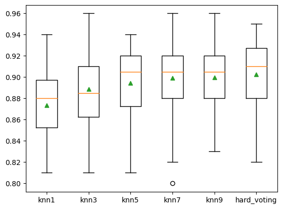
可以看到结果不断在提升。
bagging
同样,我们生成数据集后采用简单的例子来介绍bagging对应函数的用法:
 from numpy import mean

from numpy import std

from sklearn.datasets import make_classification

from sklearn.model_selection import cross_val_score

from sklearn.model_selection import RepeatedStratifiedKFold

from sklearn.ensemble import BaggingClassifier


X, y = make_classification(n_samples=1000, n_features=20, n_informative=15, n_redundant=5, random_state=5)

model = BaggingClassifier()

cv = RepeatedStratifiedKFold(n_splits=10, n_repeats=3, random_state=1)

n_scores = cross_val_score(model, X, y, scoring='accuracy', cv=cv, n_jobs=-1, error_score='raise')

print('Accuracy: %.3f (%.3f)' % (mean(n_scores), std(n_scores)))
Accuracy: 0.861 (0.042) Boosting
关于这方面的理论知识的介绍可以看我这篇博客。
这边继续关注这方面的代码怎么使用。
Adaboost
先导入各种包:
 import numpy as np

import pandas as pd

import matplotlib.pyplot as plt

plt.style.use("ggplot")

%matplotlib inline

import seaborn as sns
# 加载训练数据:
wine = pd.read_csv("https://archive.ics.uci.edu/ml/machine-learning-databases/wine/wine.data",header=None)
wine.columns = ['Class label', 'Alcohol', 'Malic acid', 'Ash', 'Alcalinity of ash','Magnesium', 'Total phenols','Flavanoids', 'Nonflavanoid phenols',
'Proanthocyanins','Color intensity', 'Hue','OD280/OD315 of diluted wines','Proline']
# 数据查看:
print("Class labels",np.unique(wine["Class label"]))
wine.head() Class labels [1 2 3] 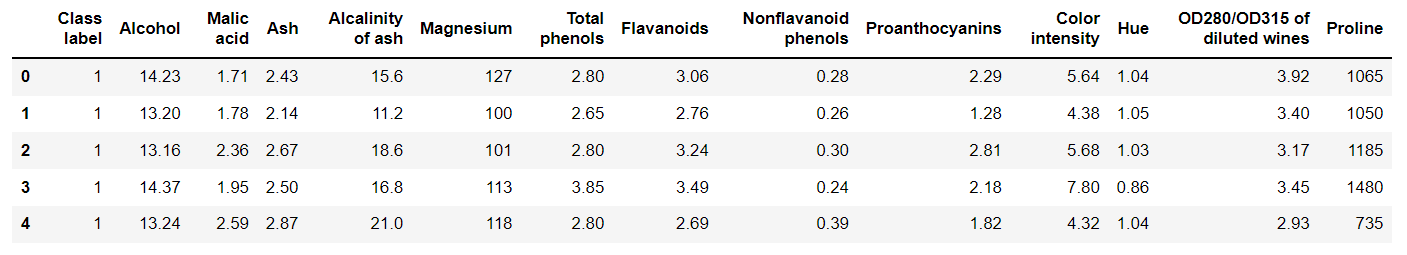
那么接下来就需要对数据进行预处理:
 # 数据预处理

# 仅仅考虑2,3类葡萄酒,去除1类

wine = wine[wine['Class label'] != 1]

y = wine['Class label'].values

X = wine[['Alcohol','OD280/OD315 of diluted wines']].values


# 将分类标签变成二进制编码:

from sklearn.preprocessing import LabelEncoder

le = LabelEncoder()

y = le.fit_transform(y)


# 按8:2分割训练集和测试集

from sklearn.model_selection import train_test_split

X_train,X_test,y_train,y_test = train_test_split(X,y,test_size=0.2,random_state=1,stratify=y)  # stratify参数代表了按照y的类别等比例抽样
这里补充一下LabelEncoder的用法,官方给出的最简洁的解释为:
Encode labels with value between 0 and n_classes-1.
也就是可以将原来的标签约束到[0,n_classes-1]之间,1个数字代表一个类别。其具体的方法为:
-
fit、transform:
 le = LabelEncoder()

le = le.fit(['A','B','C'])  # 使用le去拟合所有标签

data = le.transform(data) # 将原来的标签转换为编码 -
fit_transform:
 le = LabelEncoder()

data = le.fit_transform(data) -
inverse_transform:根据编码反向推出原来类别标签
 le.inverse_transform([0,1,2])

# 输出['A','B','C']
继续AdaBoost。
我们接下来对比一下单一决策树和集成之间的效果差异。
 # 使用单一决策树建模

from sklearn.tree import DecisionTreeClassifier

tree = DecisionTreeClassifier(criterion='entropy',random_state=1,max_depth=1)

from sklearn.metrics import accuracy_score

tree = tree.fit(X_train,y_train)

y_train_pred = tree.predict(X_train)

y_test_pred = tree.predict(X_test)

tree_train = accuracy_score(y_train,y_train_pred)

tree_test = accuracy_score(y_test,y_test_pred)

print('Decision tree train/test accuracies %.3f/%.3f' % (tree_train,tree_test))
Decision tree train/test accuracies 0.916/0.875 下面对AdaBoost进行建模:
 from sklearn.ensemble import AdaBoostClassifier

ada = AdaBoostClassifier(base_estimator=tree,  # 基分类器

                         n_estimators=500, # 最大迭代次数

                        learning_rate=0.1,

                        random_state= 1)

ada.fit(X_train, y_train)

y_train_pred = ada.predict(X_train)

y_test_pred = ada.predict(X_test)

ada_train = accuracy_score(y_train,y_train_pred)

ada_test = accuracy_score(y_test,y_test_pred)

print('Adaboost train/test accuracies %.3f/%.3f' % (ada_train,ada_test))
Adaboost train/test accuracies 1.000/0.917 可以看见分类精度提升了不少,下面我们可以观察他们的决策边界有什么不同:
 x_min = X_train[:, 0].min() - 1

x_max = X_train[:, 0].max() + 1

y_min = X_train[:, 1].min() - 1

y_max = X_train[:, 1].max() + 1

xx, yy = np.meshgrid(np.arange(x_min, x_max, 0.1),np.arange(y_min, y_max, 0.1))

f, axarr = plt.subplots(nrows=1, ncols=2,sharex='col',sharey='row',figsize=(12, 6))

for idx, clf, tt in zip([0, 1],[tree, ada],['Decision tree', 'Adaboost']):

    clf.fit(X_train, y_train)

    Z = clf.predict(np.c_[xx.ravel(), yy.ravel()])

    Z = Z.reshape(xx.shape)

    axarr[idx].contourf(xx, yy, Z, alpha=0.3)

    axarr[idx].scatter(X_train[y_train==0, 0],X_train[y_train==0, 1],c='blue', marker='^')

    axarr[idx].scatter(X_train[y_train==1, 0],X_train[y_train==1, 1],c='red', marker='o')

    axarr[idx].set_title(tt)

axarr[0].set_ylabel('Alcohol', fontsize=12)

plt.tight_layout()

plt.text(0, -0.2,s='OD280/OD315 of diluted wines',ha='center',va='center',fontsize=12,transform=axarr[1].transAxes)

plt.show() 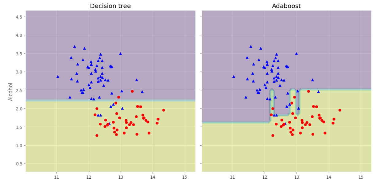
可以看淡AdaBoost的决策边界比单个决策树的决策边界复杂很多。
梯度提升GBDT
这里的理论解释用我对西瓜书的学习笔记吧:
GBDT是一种迭代的决策树算法,由多个决策树组成,所有树的结论累加起来作为最终答案。接下来从这两个方面进行介绍: Regression Decision Tree(回归树)、Gradient Boosting(梯度提升)、Shrinkage
DT
先补充一下决策树的类别,包含两种:
- 分类决策树 :用于预测分类标签值,例如天气的类型、用户的性别等
- 回归决策树 :用来预测连续实数值,例如天气温度、用户年龄
这两者的重要区别在于 回归决策树的输出结果可以相加,分类决策树的输出结果不可以相加 ,例如回归决策树分别输出10岁、5岁、2岁,那他们相加得到17岁,可以作为结果使用;但是分类决策树分别输出男、男、女,这样的结果是无法进行相加处理的。因此 GBDT中的树都是回归树,GBDT的核心在于累加所有树的结果作为最终结果 。
回归树,救赎用树模型来做回归问题,其 每一片叶子都输出一个预测值 ,而这个预测值一般是 该片叶子所含训练集元素输出的均值 ,即 \(c_m=ave(y_i\mid x_i \in leaf_m)\)
一般来说常见的回归决策树为CART,因此下面先介绍CART如何应用于回归问题。
在回归问题中,CART主要 使用均方误差(mse)或者平均绝对误差(mae)来作为选择特征以及选择划分点时的依据 。因此用于回归问题时,目标就是要 构建出一个函数 \(f(x)\) 能够有效地拟合数据集 \(D\) (样本数为n)中的元素,使得所选取的度量指标最小 ,例如取mse,即:
\]
而对于构建好的CART回归树来说,假设其存在 \(M\) 片叶子,那么其mse的公式可以写成:
\]
其中 \(R_m\) 代表第 \(m\) 片叶子,而 \(c_m\) 代表第 \(m\) 片叶子的预测值。
要使得最小化mse,就需要对每一片叶子的mse都进行最小化。由统计学的知识可知道,只需要使**每片叶子的预测值为该片叶子中含有的训练元素的均值即可,即 \(c_m=ave(y_i\mid x_i \in leaf_m)\) 。
因此CART的学习方法就是 遍历每一个变量且遍历变量中的每一个切分点,寻找能够使得mse最小的切分变量和切分点 ,即最小化如下公式:
\]
另外一个值得了解的想法就是 为什么CART必须是二叉树 ,其实是因为如果划分结点增多,即划分出来的区间也增多, 遍历的难度加大 。而如果想要细分为多个区域,实际上只需要让CART回归树的层次更深即可,这样遍历难度将小很多。
Gradient Boosting
梯度提升算法的流程与AdaBoost有点类似,而区别在于 AdaBoost的特点在于每一轮是对分类正确和错误的样本分别进行修改权重 ,而 梯度提升算法的每一轮学习都是为了减少上一轮的误差 ,具体可以看以下算法描述:
Step1、给定训练数据集T及损失函数L,这里可以认为损失函数为mse
Step2、初始化:
\]
上式求解出来为:
\]
Step3、目标基分类器(回归树)数目为 \(M\) ,对于 \(m=1,2,...M\) :
(1)、对于 \(i=1,2,...N\) ,计算
\]
(2)、对 \(r_{mi}\) 进行拟合学习得到一个回归树,其叶结点区域为 \(R_{mj},j=1,2,...J\)
(3)、对 \(j=1,2,...J\) ,计算该对应叶结点 \(R_{mj}\) 的输出预测值:
\]
(4)、更新 \(f_m(x)=f_{m-1}(x)+\sum _{j=1}^{J}c_{mj}I(x \in R_{mj})\)
Step4、得到回归树:
\]
为什么损失函数的负梯度能够作为回归问题残差的近似值呢? :因为对于损失函数为mse来说, 其求导的结果其实就是预测值与真实值之间的差值,那么负梯度也就是我们预测的残差 \((y_i - f(x_i))\) ,因此 只要下一个回归树对负梯度进行拟合再对多个回归树进行累加,就可以更好地逼近真实值 。
Shrinkage
Shrinkage是一种用来 对GBDT进行优化,防止其陷入过拟合的方法 ,其具体思想是: 减少每一次迭代对于残差的收敛程度或者逼近程度 ,也就是说该思想认为迭代时 每一次少逼近一些,然后迭代次数多一些的效果,比每一次多逼近一些,然后迭代次数少一些的效果要更好 。那么具体的实现就是 在每个回归树的累加前乘上学习率 ,即:
\]
建模实现
下面对GBDT的模型进行解释以及建模实现。
引入相关库:
 from sklearn.metrics import mean_squared_error

from sklearn.datasets import make_friedman1

from sklearn.ensemble import GradientBoostingRegressor
GBDT还有一个做分类的模型是GradientBoostingClassifier。
下面整理一下模型的各个参数:
| 参数名称 | 参数意义 |
|---|---|
| loss | {‘ls’, ‘lad’, ‘huber’, ‘quantile’}, default=’ls’:‘ls’ 指最小二乘回归. ‘lad’是最小绝对偏差,是仅基于输入变量的顺序信息的高度鲁棒的损失函数;‘huber’ 是两者的结合 |
| quantile | 允许分位数回归(用于alpha指定分位数) |
| learning_rate | 学习率缩小了每棵树的贡献learning_rate。在learning_rate和n_estimators之间需要权衡。 |
| n_estimators | 要执行的提升次数,可以认为是基分类器的数目 |
| subsample | 用于拟合各个基础学习者的样本比例。如果小于1.0,则将导致随机梯度增强 |
| criterion | {'friedman_mse','mse','mae'},默认='friedman_mse':“ mse”是均方误差,“ mae”是平均绝对误差。默认值“ friedman_mse”通常是最好的,因为在某些情况下它可以提供更好的近似值。 |
| min_samples_split | 拆分内部节点所需的最少样本数 |
| min_samples_leaf | 在叶节点处需要的最小样本数 |
| min_weight_fraction_leaf | 在所有叶节点处(所有输入样本)的权重总和中的最小加权分数。如果未提供sample_weight,则样本的权重相等。 |
| max_depth | 各个回归模型的最大深度。最大深度限制了树中节点的数量。调整此参数以获得最佳性能;最佳值取决于输入变量的相互作用 |
| min_impurity_decrease | 如果节点分裂会导致杂质(损失函数)的减少大于或等于该值,则该节点将被分裂 |
| min_impurity_split | 提前停止树木生长的阈值。如果节点的杂质高于阈值,则该节点将分裂 |
| max_features | {‘auto’, ‘sqrt’, ‘log2’},int或float:寻找最佳分割时要考虑的功能数量 |
可能各个参数一开始难以理解,但是随着使用会加深印象的。
 X, y = make_friedman1(n_samples=1200, random_state=0, noise=1.0)

X_train, X_test = X[:200], X[200:]

y_train, y_test = y[:200], y[200:]

est = GradientBoostingRegressor(n_estimators=100, learning_rate=0.1,

    max_depth=1, random_state=0, loss='ls').fit(X_train, y_train)

mean_squared_error(y_test, est.predict(X_test))
5.009154859960321 from sklearn.datasets import make_regression
from sklearn.ensemble import GradientBoostingRegressor
from sklearn.model_selection import train_test_split
X, y = make_regression(random_state=0)
X_train, X_test, y_train, y_test = train_test_split(
X, y, random_state=0)
reg = GradientBoostingRegressor(random_state=0)
reg.fit(X_train, y_train)
reg.score(X_test, y_test) XGBoost
关于XGBoost的理论,其实它跟GBDT差不多,只不过在泰勒展开时考虑了二阶导函数,并在库实现中增加了很多的优化。而关于其参数的设置也相当复杂,因此这里简单介绍其用法即可。
安装XGBoost
pip install xgboost 数据接口
xgboost库所使用的数据类型为特殊的DMatrix类型,因此其读入文件比较特殊:
 # 1.LibSVM文本格式文件

dtrain = xgb.DMatrix('train.svm.txt')

dtest = xgb.DMatrix('test.svm.buffer')

# 2.CSV文件(不能含类别文本变量,如果存在文本变量请做特征处理如one-hot)

dtrain = xgb.DMatrix('train.csv?format=csv&label_column=0')

dtest = xgb.DMatrix('test.csv?format=csv&label_column=0')

# 3.NumPy数组

data = np.random.rand(5, 10)  # 5 entities, each contains 10 features

label = np.random.randint(2, size=5)  # binary target

dtrain = xgb.DMatrix(data, label=label)

# 4.scipy.sparse数组

csr = scipy.sparse.csr_matrix((dat, (row, col)))

dtrain = xgb.DMatrix(csr)

# pandas数据框dataframe

data = pandas.DataFrame(np.arange(12).reshape((4,3)), columns=['a', 'b', 'c'])

label = pandas.DataFrame(np.random.randint(2, size=4))

dtrain = xgb.DMatrix(data, label=label)
第一次读入后可以先保存为对应的二进制文件方便下次读取:
 # 1.保存DMatrix到XGBoost二进制文件中

dtrain = xgb.DMatrix('train.svm.txt')

dtrain.save_binary('train.buffer')

# 2. 缺少的值可以用DMatrix构造函数中的默认值替换:

dtrain = xgb.DMatrix(data, label=label, missing=-999.0)

# 3.可以在需要时设置权重:

w = np.random.rand(5, 1)

dtrain = xgb.DMatrix(data, label=label, missing=-999.0, weight=w)
参数设置
 import pandas as pd

df_wine = pd.read_csv('https://archive.ics.uci.edu/ml/machine-learning-databases/wine/wine.data',header=None)

df_wine.columns = ['Class label', 'Alcohol','Malic acid', 'Ash','Alcalinity of ash','Magnesium', 'Total phenols',

                   'Flavanoids', 'Nonflavanoid phenols','Proanthocyanins','Color intensity', 'Hue','OD280/OD315 of diluted wines','Proline']

df_wine = df_wine[df_wine['Class label'] != 1]  # drop 1 class

y = df_wine['Class label'].values

X = df_wine[['Alcohol','OD280/OD315 of diluted wines']].values

from sklearn.model_selection import train_test_split  # 切分训练集与测试集

from sklearn.preprocessing import LabelEncoder   # 标签化分类变量

import xgboost as xgb

le = LabelEncoder()

y = le.fit_transform(y)

X_train,X_test,y_train,y_test = train_test_split(X,y,test_size=0.2,

                                                 random_state=1,stratify=y)

# 构造成目标类型的数据

dtrain = xgb.DMatrix(X_train, label = y_train)

dtest = xgb.DMatrix(X_test)


# booster参数

params = {

    "booster": 'gbtree',  # 基分类器

    "objective":  "multi:softmax",  # 使用softmax

    "num_class": 10,  # 类别数

    "gamma":0.1,  # 用于控制损失函数大于gamma时就剪枝

    "max_depth": 12,  # 构造树的深度,越大越容易过拟合

    "lambda":  2,  # 用来控制正则化参数

    "subsample": 0.7,  # 随机采样70%作为训练样本

    "colsample_bytree": 0.7,  # 生成树时进行列采样,相当于随机子空间

    "min_child_weight":3,

    'verbosity':0,  # 设置成1则没有运行信息输出,设置成0则有,原文中这里的silent已经在新版本中不使用了

    "eta": 0.007,  # 相当于学习率

    "seed": 1000,  # 随机数种子

    "nthread":4,   # 线程数

    "eval_metric": "auc"

}

plst = list(params.items())  # 这里必须加上list才能够使用后续的copy
这里如果发现报错为:
Parameters: { "silent" } are not used.
那是因为参数设置中新版本已经取消了silent参数,将其更改为verbosity即可。
如果在后续中发现:
'dict_items' object has no attribute 'copy'
那是因为我们没有将items的返回变成list,像我上面那么改即可。
训练及预测
 num_round = 10

bst = xgb.train(plst, dtrain ,num_round)

# 可以加上early_stoppint_rounds = 10来设置早停机制

# 如果要指定验证集,就是

# evallist = [(deval,'eval'),(dtrain, 'train')]

# bst = xgb.train(plst, dtrain, num_round, evallist)
ypred = bst.predict(dtest) # 进行预测,跟sklearn的模型一致
xgb.plot_importance(bst) # 绘制特征重要性的图 <AxesSubplot:title={'center':'Feature importance'}, xlabel='F score', ylabel='Features'> 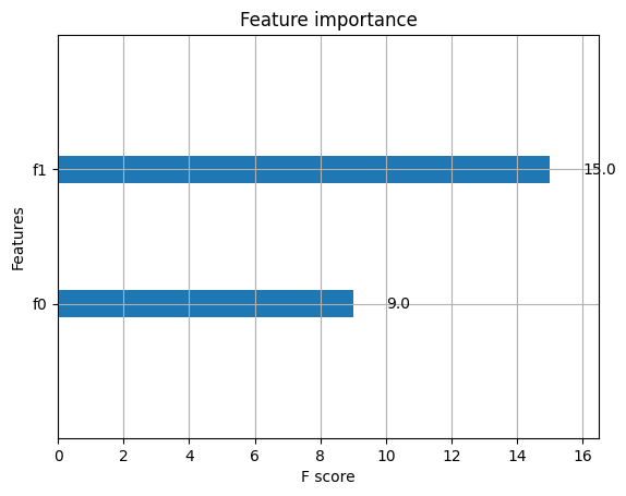
模型保存与加载
 bst.save_model("model_new_1121.model")

bst.dump_model("dump.raw.txt")

bst_new = xgb.Booster({'nthread':4})  # 先初始化参数

bst_new.load_model("model_new_1121.model")
简单算例
分类案例
 from sklearn.datasets import load_iris

import xgboost as xgb

from xgboost import plot_importance

from matplotlib import pyplot as plt

from sklearn.model_selection import train_test_split

from sklearn.metrics import accuracy_score   # 准确率

# 加载样本数据集

iris = load_iris()

X,y = iris.data,iris.target

X_train, X_test, y_train, y_test = train_test_split(X, y, test_size=0.2,

                                                    random_state=1234565) # 数据集分割

# 算法参数

params = {

    'booster': 'gbtree',

    'objective': 'multi:softmax',

    'num_class': 3,

    'gamma': 0.1,

    'max_depth': 6,

    'lambda': 2,

    'subsample': 0.7,

    'colsample_bytree': 0.75,

    'min_child_weight': 3,

    'verbosity': 0,

    'eta': 0.1,

    'seed': 1,

    'nthread': 4,

}

plst = list(params.items())

dtrain = xgb.DMatrix(X_train, y_train) # 生成数据集格式

num_rounds = 500

model = xgb.train(plst, dtrain, num_rounds) # xgboost模型训练

# 对测试集进行预测

dtest = xgb.DMatrix(X_test)

y_pred = model.predict(dtest)


# 计算准确率

accuracy = accuracy_score(y_test,y_pred)

print("accuarcy: %.2f%%" % (accuracy*100.0))


# 显示重要特征

plot_importance(model)

plt.show()
accuarcy: 96.67% 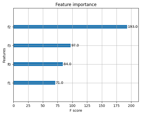
回归案例
 import xgboost as xgb

from xgboost import plot_importance

from matplotlib import pyplot as plt

from sklearn.model_selection import train_test_split

from sklearn.datasets import load_boston

from sklearn.metrics import mean_squared_error


# 加载数据集

boston = load_boston()

X,y = boston.data,boston.target


# XGBoost训练过程

X_train, X_test, y_train, y_test = train_test_split(X, y, test_size=0.2, random_state=0)


params = {

    'booster': 'gbtree',

    'objective': 'reg:squarederror',  # 设置为回归,采用平方误差

    'gamma': 0.1,

    'max_depth': 5,

    'lambda': 3,

    'subsample': 0.7,

    'colsample_bytree': 0.7,

    'min_child_weight': 3,

    'verbosity': 1,

    'eta': 0.1,

    'seed': 1000,

    'nthread': 4,

}

dtrain = xgb.DMatrix(X_train, y_train)

num_rounds = 300

plst = list(params.items())

model = xgb.train(plst, dtrain, num_rounds)

# 对测试集进行预测

dtest = xgb.DMatrix(X_test)

ans = model.predict(dtest)


# 显示重要特征

plot_importance(model)

plt.show() 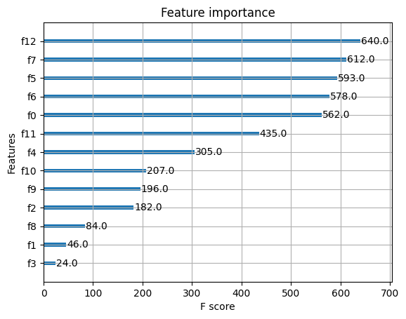
XGBoost的调参
该模型的调参一般步骤为:
- 确定学习速率和提升参数调优的初始值
- max_depth 和 min_child_weight 参数调优
- gamma参数调优
- subsample 和 colsample_bytree 参数优
- 正则化参数alpha调优
- 降低学习速率和使用更多的决策树
可以使用网格搜索来进行调优:
 import xgboost as xgb

import pandas as pd

from sklearn.model_selection import train_test_split

from sklearn.model_selection import GridSearchCV

from sklearn.metrics import roc_auc_score


iris = load_iris()

X,y = iris.data,iris.target

col = iris.target_names

train_x, valid_x, train_y, valid_y = train_test_split(X, y, test_size=0.3, random_state=1)   # 分训练集和验证集

parameters = {

              'max_depth': [5, 10, 15, 20, 25],

              'learning_rate': [0.01, 0.02, 0.05, 0.1, 0.15],

              'n_estimators': [500, 1000, 2000, 3000, 5000],

              'min_child_weight': [0, 2, 5, 10, 20],

              'max_delta_step': [0, 0.2, 0.6, 1, 2],

              'subsample': [0.6, 0.7, 0.8, 0.85, 0.95],

              'colsample_bytree': [0.5, 0.6, 0.7, 0.8, 0.9],

              'reg_alpha': [0, 0.25, 0.5, 0.75, 1],

              'reg_lambda': [0.2, 0.4, 0.6, 0.8, 1],

              'scale_pos_weight': [0.2, 0.4, 0.6, 0.8, 1]


}


xlf = xgb.XGBClassifier(max_depth=10,

            learning_rate=0.01,

            n_estimators=2000,

            silent=True,

            objective='multi:softmax',

            num_class=3 ,

            nthread=-1,

            gamma=0,

            min_child_weight=1,

            max_delta_step=0,

            subsample=0.85,

            colsample_bytree=0.7,

            colsample_bylevel=1,

            reg_alpha=0,

            reg_lambda=1,

            scale_pos_weight=1,

            seed=0,

            missing=None)

# 需要先给模型一定的初始值

gs = GridSearchCV(xlf, param_grid=parameters, scoring='accuracy', cv=3)

gs.fit(train_x, train_y)


print("Best score: %0.3f" % gs.best_score_)

print("Best parameters set: %s" % gs.best_params_ )
Best score: 0.933
Best parameters set: {'max_depth': 5} LightGBM算法
LightGBM也是像XGBoost一样,是一类集成算法,他跟XGBoost总体来说是一样的,算法本质上与Xgboost没有出入,只是在XGBoost的基础上进行了优化。
其调优过程也是一个很复杂的学问。这里就附上课程调优代码吧:
 import lightgbm as lgb

from sklearn import metrics

from sklearn.datasets import load_breast_cancer

from sklearn.model_selection import train_test_split


canceData=load_breast_cancer()

X=canceData.data

y=canceData.target

X_train,X_test,y_train,y_test=train_test_split(X,y,random_state=0,test_size=0.2)


### 数据转换

print('数据转换')

lgb_train = lgb.Dataset(X_train, y_train, free_raw_data=False)

lgb_eval = lgb.Dataset(X_test, y_test, reference=lgb_train,free_raw_data=False)


### 设置初始参数--不含交叉验证参数

print('设置参数')

params = {

          'boosting_type': 'gbdt',

          'objective': 'binary',

          'metric': 'auc',

          'nthread':4,

          'learning_rate':0.1

          }


### 交叉验证(调参)

print('交叉验证')

max_auc = float('0')

best_params = {}


# 准确率

print("调参1:提高准确率")

for num_leaves in range(5,100,5):

    for max_depth in range(3,8,1):

        params['num_leaves'] = num_leaves

        params['max_depth'] = max_depth


        cv_results = lgb.cv(

                            params,

                            lgb_train,

                            seed=1,

                            nfold=5,

                            metrics=['auc'],

                            early_stopping_rounds=10,

                            verbose_eval=True

                            )


        mean_auc = pd.Series(cv_results['auc-mean']).max()

        boost_rounds = pd.Series(cv_results['auc-mean']).idxmax()


        if mean_auc >= max_auc:

            max_auc = mean_auc

            best_params['num_leaves'] = num_leaves

            best_params['max_depth'] = max_depth

if 'num_leaves' and 'max_depth' in best_params.keys():

    params['num_leaves'] = best_params['num_leaves']

    params['max_depth'] = best_params['max_depth']


# 过拟合

print("调参2:降低过拟合")

for max_bin in range(5,256,10):

    for min_data_in_leaf in range(1,102,10):

            params['max_bin'] = max_bin

            params['min_data_in_leaf'] = min_data_in_leaf


            cv_results = lgb.cv(

                                params,

                                lgb_train,

                                seed=1,

                                nfold=5,

                                metrics=['auc'],

                                early_stopping_rounds=10,

                                verbose_eval=True

                                )


            mean_auc = pd.Series(cv_results['auc-mean']).max()

            boost_rounds = pd.Series(cv_results['auc-mean']).idxmax()


            if mean_auc >= max_auc:

                max_auc = mean_auc

                best_params['max_bin']= max_bin

                best_params['min_data_in_leaf'] = min_data_in_leaf

if 'max_bin' and 'min_data_in_leaf' in best_params.keys():

    params['min_data_in_leaf'] = best_params['min_data_in_leaf']

    params['max_bin'] = best_params['max_bin']


print("调参3:降低过拟合")

for feature_fraction in [0.6,0.7,0.8,0.9,1.0]:

    for bagging_fraction in [0.6,0.7,0.8,0.9,1.0]:

        for bagging_freq in range(0,50,5):

            params['feature_fraction'] = feature_fraction

            params['bagging_fraction'] = bagging_fraction

            params['bagging_freq'] = bagging_freq


            cv_results = lgb.cv(

                                params,

                                lgb_train,

                                seed=1,

                                nfold=5,

                                metrics=['auc'],

                                early_stopping_rounds=10,

                                verbose_eval=True

                                )


            mean_auc = pd.Series(cv_results['auc-mean']).max()

            boost_rounds = pd.Series(cv_results['auc-mean']).idxmax()


            if mean_auc >= max_auc:

                max_auc=mean_auc

                best_params['feature_fraction'] = feature_fraction

                best_params['bagging_fraction'] = bagging_fraction

                best_params['bagging_freq'] = bagging_freq


if 'feature_fraction' and 'bagging_fraction' and 'bagging_freq' in best_params.keys():

    params['feature_fraction'] = best_params['feature_fraction']

    params['bagging_fraction'] = best_params['bagging_fraction']

    params['bagging_freq'] = best_params['bagging_freq']


print("调参4:降低过拟合")

for lambda_l1 in [1e-5,1e-3,1e-1,0.0,0.1,0.3,0.5,0.7,0.9,1.0]:

    for lambda_l2 in [1e-5,1e-3,1e-1,0.0,0.1,0.4,0.6,0.7,0.9,1.0]:

        params['lambda_l1'] = lambda_l1

        params['lambda_l2'] = lambda_l2

        cv_results = lgb.cv(

                            params,

                            lgb_train,

                            seed=1,

                            nfold=5,

                            metrics=['auc'],

                            early_stopping_rounds=10,

                            verbose_eval=True

                            )


        mean_auc = pd.Series(cv_results['auc-mean']).max()

        boost_rounds = pd.Series(cv_results['auc-mean']).idxmax()


        if mean_auc >= max_auc:

            max_auc=mean_auc

            best_params['lambda_l1'] = lambda_l1

            best_params['lambda_l2'] = lambda_l2

if 'lambda_l1' and 'lambda_l2' in best_params.keys():

    params['lambda_l1'] = best_params['lambda_l1']

    params['lambda_l2'] = best_params['lambda_l2']


print("调参5:降低过拟合2")

for min_split_gain in [0.0,0.1,0.2,0.3,0.4,0.5,0.6,0.7,0.8,0.9,1.0]:

    params['min_split_gain'] = min_split_gain


    cv_results = lgb.cv(

                        params,

                        lgb_train,

                        seed=1,

                        nfold=5,

                        metrics=['auc'],

                        early_stopping_rounds=10,

                        verbose_eval=True

                        )


    mean_auc = pd.Series(cv_results['auc-mean']).max()

    boost_rounds = pd.Series(cv_results['auc-mean']).idxmax()


    if mean_auc >= max_auc:

        max_auc=mean_auc


        best_params['min_split_gain'] = min_split_gain

if 'min_split_gain' in best_params.keys():

    params['min_split_gain'] = best_params['min_split_gain']


print(best_params)
{'bagging_fraction': 0.7,
'bagging_freq': 30,
'feature_fraction': 0.8,
'lambda_l1': 0.1,
'lambda_l2': 0.0,
'max_bin': 255,
'max_depth': 4,
'min_data_in_leaf': 81,
'min_split_gain': 0.1,
'num_leaves': 10} Blending与Stacking
Stacking,这个集成方法在比赛中被称为“懒人”算法,因为它不需要花费过多时间的调参就可以得到一个效果不错的算法。
Stacking集成算法可以理解为一个两层的集成,第一层含有多个基础分类器,把预测的结果(元特征)提供给第二层, 而第二层的分类器通常是逻辑回归,他把一层分类器的结果当做特征做拟合输出预测结果。
而Blending就是简化版的Stacking,因此我们先对前者进行介绍。
Blending集成学习算法
算法流程
Blending的算法流程为:
- 将数据集划分为训练集与测试集,训练集再划分为训练集与验证集
- 创建第一层的多个模型(可同质也可异质),然后对训练集进行学习
- 第一层的模型训练完成后对验证集和测试集做出预测,假设K个模型,那么就得到 \(A_1,...,A_K\) 和 \(B_1,...,B_K\) ,其中每个代表一个基分类器对验证集或测试集的所有结果输出。
- 创建第二层的分类器,其将 \(A_1,...,A_K\) 作为训练数据集,那么样本数目就是验证集的样本数目,特征数目就是K,将真实的验证集标签作为标签,从而来训练该分类器
- 对测试集的预测则是将 \(B_1,...,B_K\) 作为特征,用第二层的分类器进行预测。
具体实现
具体的实现如下:
 import numpy as np

import pandas as pd

import matplotlib.pyplot as plt

plt.style.use("ggplot")

%matplotlib inline

import seaborn as sns

# 创建数据

from sklearn import datasets

from sklearn.datasets import make_blobs

from sklearn.model_selection import train_test_split

data, target = make_blobs(n_samples=10000, centers=2, random_state=1, cluster_std=1.0 )

## 创建训练集和测试集

X_train1,X_test,y_train1,y_test = train_test_split(data, target, test_size=0.2, random_state=1)

## 创建训练集和验证集

X_train,X_val,y_train,y_val = train_test_split(X_train1, y_train1, test_size=0.3, random_state=1)

print("The shape of training X:",X_train.shape)

print("The shape of training y:",y_train.shape)

print("The shape of test X:",X_test.shape)

print("The shape of test y:",y_test.shape)

print("The shape of validation X:",X_val.shape)

print("The shape of validation y:",y_val.shape)
The shape of training X: (5600, 2)
The shape of training y: (5600,)
The shape of test X: (2000, 2)
The shape of test y: (2000,)
The shape of validation X: (2400, 2)
The shape of validation y: (2400,) # 设置第一层分类器
from sklearn.svm import SVC
from sklearn.ensemble import RandomForestClassifier
from sklearn.neighbors import KNeighborsClassifier
clfs = [SVC(probability = True),RandomForestClassifier(n_estimators=5, n_jobs=-1, criterion='gini'),KNeighborsClassifier()]
# 设置第二层分类器
from sklearn.linear_model import LinearRegression
lr = LinearRegression()
# 输出第一层的验证集结果与测试集结果
val_features = np.zeros((X_val.shape[0],len(clfs))) # 初始化验证集结果
test_features = np.zeros((X_test.shape[0],len(clfs))) # 初始化测试集结果
for i,clf in enumerate(clfs):
clf.fit(X_train,y_train)
# porba函数得到的是对于每个类别的预测分数,取出第一列代表每个样本为第一类的概率
val_feature = clf.predict_proba(X_val)[:, 1]
test_feature = clf.predict_proba(X_test)[:,1]
val_features[:,i] = val_feature
test_features[:,i] = test_feature
# 将第一层的验证集的结果输入第二层训练第二层分类器
lr.fit(val_features,y_val)
# 输出预测的结果
from sklearn.model_selection import cross_val_score
cross_val_score(lr,test_features,y_test,cv=5) array([1., 1., 1., 1., 1.]) 可以看到交叉验证的结果很好。
对于小作业我总有些疑问,那就是这个iris数据的特征为4,然后预测类别数为3,那么首先是特征为4超过3维度,应该怎么决策边界,难道舍弃一些维度吗?其次是类别数为3,那么在计算的时候取的是[;1]也就是类别为1的概率,那么只取这个作为下一层的特征是否足够,因为类别为0和类别为2的概率完全舍弃的话不行吧。
Stacking
算法流程
下面这张图可以很好的理解流程:
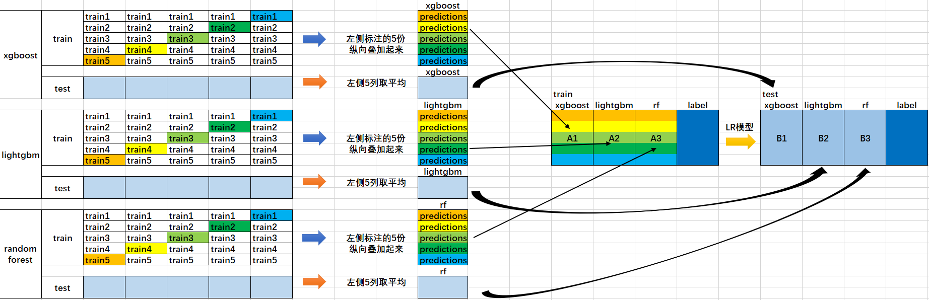
- 首先将所有数据划分测试集和训练集,假设训练集总共有10000行,测试集总共2500行,对第一层的分类器进行5折交叉验证,那么验证集就划分为2000行,训练集为8000行。
- 每次验证就相当于使用8000条训练数据去训练模型然后用2000条验证数据去验证, 并且每一次都将训练出来的模型对测试集的2500条数据进行预测 ,那么经过5次交叉验证,对于每个基分类器可以得到中间的 \(5\times 2000\) 的五份验证集数据,以及 \(5\times 2500\) 的五份测试集的预测结果
- 接下来将验证集拼成10000行长的矩阵,记为 \(A_1\) (对于第1个基分类器),而对于 \(5\times 2500\) 行的测试集的预测结果进行加权平均,得到2500行1列的矩阵,记为 \(B_1\)
- 那么假设这里是3个基分类器,因此有 \(A_1,A_2,A_3,B_1,B_2,B_3\) 六个矩阵,接下来将 \(A_1,A_2,A_3\) 矩阵拼成10000行3列的矩阵作为训练数据集,而验证集的真实标签作为训练数据的标签;将 \(B_1,B_2,B_3\) 拼成2500行3列的矩阵作为测试数据集合。
- 那么对下层的学习器进行训练
具体代码
 from sklearn import datasets

iris = datasets.load_iris()

X, y = iris.data[:, 1:3], iris.target  # 只取出两个特征

from sklearn.model_selection import cross_val_score

from sklearn.linear_model import LogisticRegression

from sklearn.neighbors import KNeighborsClassifier

from sklearn.naive_bayes import GaussianNB

from sklearn.ensemble import RandomForestClassifier

from mlxtend.classifier import StackingCVClassifier


RANDOM_SEED = 42


clf1 = KNeighborsClassifier(n_neighbors = 1)

clf2 = RandomForestClassifier(random_state = RANDOM_SEED)

clf3 = GaussianNB()

lr = LogisticRegression()


sclf = StackingCVClassifier(classifiers = [clf1, clf2, clf3],  # 第一层的分类器

                           meta_classifier = lr,  # 第二层的分类器

                           random_state = RANDOM_SEED)

print("3折交叉验证:\n")

for clf, label in zip([clf1, clf2, clf3, sclf], ['KNN','RandomForest','Naive Bayes',

                                                'Stack']):

    scores = cross_val_score(clf, X, y, cv = 3, scoring = 'accuracy')

    print("Accuracy: %0.2f (+/- %0.2f) [%s]" % (scores.mean(), scores.std(), label))
3折交叉验证:
Accuracy: 0.91 (+/- 0.01) [KNN]
Accuracy: 0.95 (+/- 0.01) [RandomForest]
Accuracy: 0.91 (+/- 0.02) [Naive Bayes]
Accuracy: 0.93 (+/- 0.02) [Stack] 接下来尝试将决策边界画出:
 from mlxtend.plotting import plot_decision_regions

import matplotlib.gridspec as gridspec

import itertools


gs = gridspec.GridSpec(2,2)

# 可以理解为将子图划分为了2*2的区域

fig = plt.figure(figsize = (10,8))


for clf, lab, grd in zip([clf1, clf2, clf3, sclf], ['KNN',

                                                    'RandomForest',

                                                    'Naive Bayes',

                                                    'Stack'],

                        itertools.product([0,1],repeat=2)):

    clf.fit(X, y)

    ax = plt.subplot(gs[grd[0],grd[1]])

    # grd依次为(0,0),(0,1),(1,0),(1,1),那么传入到gs中就可以得到指定的区域

    fig = plot_decision_regions(X = X, y = y, clf = clf)

    plt.title(lab)


plt.show() 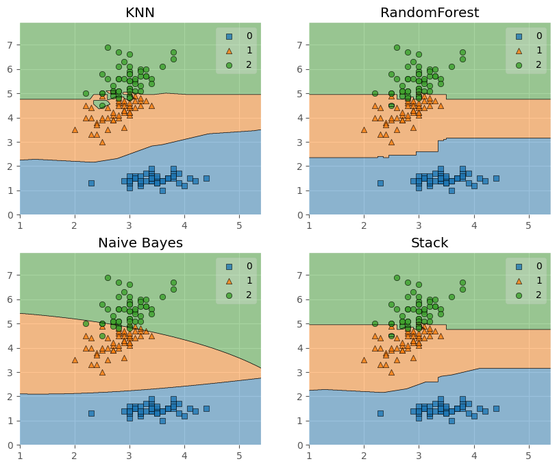
这里补充两个第一次见到的函数:
-
itertools.product([0,1],repeat = 2):该模块下的product函数一般是传进入两个集合,例如传进入[0,1],[1,2]然后返回[(0,1),(0,2),(1,1),(1,2)],那么这里只传进去一个参数然后repeat=2相当于传进去[0,1],[0,1],产生[(0,0),(0,1),(1,0),(1,1)],如果repeat=3就是
 (0, 0, 0)

(0, 0, 1)

(0, 1, 0)

(0, 1, 1)

(1, 0, 0)

(1, 0, 1)

(1, 1, 0)

(1, 1, 1) -
gs = gridspec.GridSpec(2,2):这个函数相当于我将子图划分为2*2总共4个区域,那么在下面subplot中就可以例如调用gs[0,1]来获取(0,1)这个区域,下面的例子或者更好理解:
 plt.figure()


gs=gridspec.GridSpec(3,3)#分为3行3列

ax1=plt.subplot(gs[0,:])

ax1=plt.subplot(gs[1,:2])

ax1=plt.subplot(gs[1:,2])

ax1=plt.subplot(gs[-1,0])

ax1=plt.subplot(gs[-1,-2])
继续回到Stacking中。
前面我们是使用第一层的分类器其输出作为第二层的输入,那么如果希望使用第一层所有基分类器所产生的的类别概率值作为第二层分类器的数目,需要在StackingClassifier 中增加一个参数设置:use_probas = True。还有一个参数设置average_probas = True,那么这些基分类器所产出的概率值将按照列被平均,否则会拼接
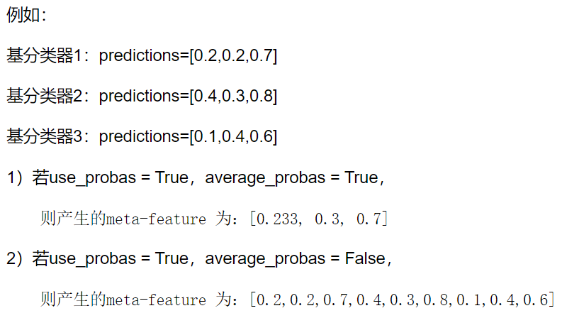
我们来进行尝试:
 clf1 = KNeighborsClassifier(n_neighbors=1)

clf2 = RandomForestClassifier(random_state=1)

clf3 = GaussianNB()

lr = LogisticRegression()


sclf = StackingCVClassifier(classifiers=[clf1, clf2, clf3],

                            use_probas=True,  #  使用概率

                            meta_classifier=lr,

                            random_state=42)


print('3折交叉验证:')


for clf, label in zip([clf1, clf2, clf3, sclf],

                      ['KNN',

                       'Random Forest',

                       'Naive Bayes',

                       'StackingClassifier']):


    scores = cross_val_score(clf, X, y, cv=3, scoring='accuracy')

    print("Accuracy: %0.2f (+/- %0.2f) [%s]"

          % (scores.mean(), scores.std(), label))
3折交叉验证:
Accuracy: 0.91 (+/- 0.01) [KNN]
Accuracy: 0.95 (+/- 0.01) [Random Forest]
Accuracy: 0.91 (+/- 0.02) [Naive Bayes]
Accuracy: 0.95 (+/- 0.02) [StackingClassifier] 另外,还可以跟网格搜索相结合:
 from sklearn.linear_model import LogisticRegression

from sklearn.neighbors import KNeighborsClassifier

from sklearn.naive_bayes import GaussianNB

from sklearn.ensemble import RandomForestClassifier

from sklearn.model_selection import GridSearchCV

from mlxtend.classifier import StackingCVClassifier


clf1 = KNeighborsClassifier(n_neighbors=1)

clf2 = RandomForestClassifier(random_state=RANDOM_SEED)

clf3 = GaussianNB()

lr = LogisticRegression()


sclf = StackingCVClassifier(classifiers=[clf1, clf2, clf3],

                            meta_classifier=lr,

                            random_state=42)


params = {'kneighborsclassifier__n_neighbors': [1, 5],

          'randomforestclassifier__n_estimators': [10, 50],

          'meta_classifier__C': [0.1, 10.0]}#

grid = GridSearchCV(estimator=sclf,  # 分类为stacking

                    param_grid=params, # 设置的参数

                    cv=5,

                    refit=True)

#最后一个参数代表在搜索参数结束后,用最佳参数结果再次fit一遍全部数据集


grid.fit(X, y)


cv_keys = ('mean_test_score', 'std_test_score', 'params')


for r,_ in enumerate(grid.cv_results_['mean_test_score']):

    print("%0.3f +/- %0.2f %r"

          % (grid.cv_results_[cv_keys[0]][r],

             grid.cv_results_[cv_keys[1]][r] / 2.0,

             grid.cv_results_[cv_keys[2]][r]))

print('Best parameters: %s' % grid.best_params_)

print('Accuracy: %.2f' % grid.best_score_)
0.947 +/- 0.03 {'kneighborsclassifier__n_neighbors': 1, 'meta_classifier__C': 0.1, 'randomforestclassifier__n_estimators': 10}
0.933 +/- 0.02 {'kneighborsclassifier__n_neighbors': 1, 'meta_classifier__C': 0.1, 'randomforestclassifier__n_estimators': 50}
0.940 +/- 0.02 {'kneighborsclassifier__n_neighbors': 1, 'meta_classifier__C': 10.0, 'randomforestclassifier__n_estimators': 10}
0.940 +/- 0.02 {'kneighborsclassifier__n_neighbors': 1, 'meta_classifier__C': 10.0, 'randomforestclassifier__n_estimators': 50}
0.953 +/- 0.02 {'kneighborsclassifier__n_neighbors': 5, 'meta_classifier__C': 0.1, 'randomforestclassifier__n_estimators': 10}
0.953 +/- 0.02 {'kneighborsclassifier__n_neighbors': 5, 'meta_classifier__C': 0.1, 'randomforestclassifier__n_estimators': 50}
0.953 +/- 0.02 {'kneighborsclassifier__n_neighbors': 5, 'meta_classifier__C': 10.0, 'randomforestclassifier__n_estimators': 10}
0.953 +/- 0.02 {'kneighborsclassifier__n_neighbors': 5, 'meta_classifier__C': 10.0, 'randomforestclassifier__n_estimators': 50}
Best parameters: {'kneighborsclassifier__n_neighbors': 5, 'meta_classifier__C': 0.1, 'randomforestclassifier__n_estimators': 10}
Accuracy: 0.95 而如果希望在算法中多次使用某个模型,就可以在参数网格中添加一个附加的数字后缀:
 params = {'kneighborsclassifier-1__n_neighbors': [1, 5],

          'kneighborsclassifier-2__n_neighbors': [1, 5],

          'randomforestclassifier__n_estimators': [10, 50],

          'meta_classifier__C': [0.1, 10.0]}
我们还可以结合随机子空间的思想,为Stacking第一层的不同子模型设置不同的特征:
 from sklearn.datasets import load_iris

from mlxtend.classifier import StackingCVClassifier

from mlxtend.feature_selection import ColumnSelector

from sklearn.pipeline import make_pipeline

from sklearn.linear_model import LogisticRegression


iris = load_iris()

X = iris.data

y = iris.target


pipe1 = make_pipeline(ColumnSelector(cols=(0, 2)),  # 选择第0,2列

                      LogisticRegression())  # 可以理解为先挑选特征再以基分类器为逻辑回归

pipe2 = make_pipeline(ColumnSelector(cols=(1, 2, 3)),  # 选择第1,2,3列

                      LogisticRegression())  # 两个基分类器都是逻辑回归

sclf = StackingCVClassifier(classifiers=[pipe1, pipe2],

                            # 两个基分类器区别在于使用特征不同

                            meta_classifier=LogisticRegression(),

                            random_state=42)


sclf.fit(X, y) 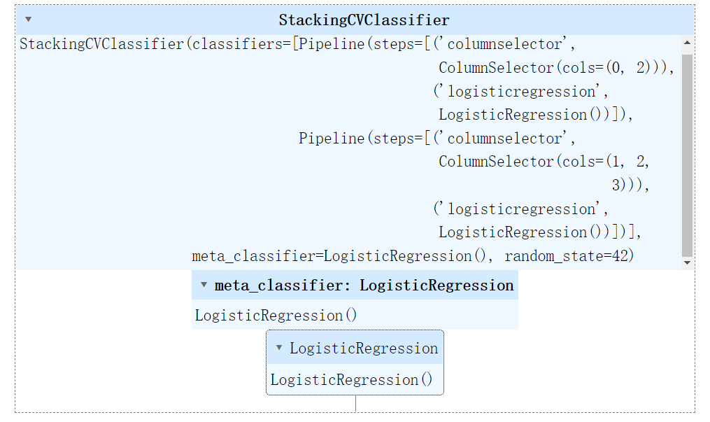
下面我们可以画ROC曲线:
 from sklearn import model_selection

from sklearn.linear_model import LogisticRegression

from sklearn.neighbors import KNeighborsClassifier

from sklearn.svm import SVC

from sklearn.ensemble import RandomForestClassifier

from mlxtend.classifier import StackingCVClassifier

from sklearn.metrics import roc_curve, auc

from sklearn.model_selection import train_test_split

from sklearn import datasets

from sklearn.preprocessing import label_binarize

from sklearn.multiclass import OneVsRestClassifier


iris = datasets.load_iris()

X, y = iris.data[:, [0, 1]], iris.target  # 只用了前两个特征


y = label_binarize(y, classes = [0,1,2])

# 因为y里面有三个类别,分类标注为0,1,2,这里是将y变换为一个n*3的矩阵

# 每一行为3代表类别数目为3,然后如果y是第0类就是100,第一类就是010,第二类就是001

# 关键在于后面的classes如何制定,如果是[0,2,1]那么是第二类就是010,第一类是001

n_classes = y.shape[1]


RANDOM_SEED = 42


X_train, X_test, y_train, y_test = train_test_split(X, y, test_size=0.33,

                                                    random_state=RANDOM_SEED)


clf1 =  LogisticRegression()

clf2 = RandomForestClassifier(random_state=RANDOM_SEED)

clf3 = SVC(random_state=RANDOM_SEED)

lr = LogisticRegression()


sclf = StackingCVClassifier(classifiers=[clf1, clf2, clf3],

                            meta_classifier=lr)


classifier = OneVsRestClassifier(sclf)

# 这个对象在拟合时会对每一类学习一个分类器,用来做二分类,分别该类和其他所有类

y_score = classifier.fit(X_train, y_train).decision_function(X_test)

# decision_function是预测X_test在决策边界的哪一边,然后距离有多大,可以认为是评估指标

# Compute ROC curve and ROC area for each class

fpr = dict()

tpr = dict()

roc_auc = dict()

for i in range(n_classes):

    fpr[i], tpr[i], _ = roc_curve(y_test[:, i], y_score[:, i])

    roc_auc[i] = auc(fpr[i], tpr[i])


# Compute micro-average ROC curve and ROC area

fpr["micro"], tpr["micro"], _ = roc_curve(y_test.ravel(), y_score.ravel())

roc_auc["micro"] = auc(fpr["micro"], tpr["micro"])


plt.figure()

lw = 2

plt.plot(fpr[2], tpr[2], color='darkorange',

         lw=lw, label='ROC curve (area = %0.2f)' % roc_auc[2])

plt.plot([0, 1], [0, 1], color='navy', lw=lw, linestyle='--')

plt.xlim([0.0, 1.0])

plt.ylim([0.0, 1.05])

plt.xlabel('False Positive Rate')

plt.ylabel('True Positive Rate')

plt.title('Receiver operating characteristic example')

plt.legend(loc="lower right")

plt.show() 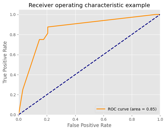
集成学习案例1——幸福感预测
背景介绍
此案例是一个数据挖掘类型的比赛——幸福感预测的baseline。比赛的数据使用的是官方的《中国综合社会调查(CGSS)》文件中的调查结果中的数据,其共包含有139个维度的特征,包括个体变量(性别、年龄、地域、职业、健康、婚姻与政治面貌等等)、家庭变量(父母、配偶、子女、家庭资本等等)、社会态度(公平、信用、公共服务)等特征。赛题要求使用以上 139 维的特征,使用 8000 余组数据进行对于个人幸福感的预测(预测值为1,2,3,4,5,其中1代表幸福感最低,5代表幸福感最高)
具体代码
导入需要的包
 import os

import time

import pandas as pd

import numpy as np

import seaborn as sns

from sklearn.linear_model import LogisticRegression

from sklearn.svm import SVC, LinearSVC

from sklearn.ensemble import RandomForestClassifier

from sklearn.neighbors import KNeighborsClassifier

from sklearn.naive_bayes import GaussianNB

from sklearn.linear_model import Perceptron

from sklearn.linear_model import SGDClassifier

from sklearn.tree import DecisionTreeClassifier

from sklearn import metrics

from datetime import datetime

import matplotlib.pyplot as plt

from sklearn.metrics import roc_auc_score, roc_curve, mean_squared_error,mean_absolute_error, f1_score

import lightgbm as lgb

import xgboost as xgb

from sklearn.ensemble import RandomForestRegressor as rfr

from sklearn.ensemble import ExtraTreesRegressor as etr

from sklearn.linear_model import BayesianRidge as br

from sklearn.ensemble import GradientBoostingRegressor as gbr

from sklearn.linear_model import Ridge

from sklearn.linear_model import Lasso

from sklearn.linear_model import LinearRegression as lr

from sklearn.linear_model import ElasticNet as en

from sklearn.kernel_ridge import KernelRidge as kr

from sklearn.model_selection import  KFold, StratifiedKFold,GroupKFold, RepeatedKFold

from sklearn.model_selection import train_test_split

from sklearn.model_selection import GridSearchCV

from sklearn import preprocessing

import logging

import warnings


warnings.filterwarnings('ignore') #消除warning
导入数据集
 train = pd.read_csv("train.csv", parse_dates=['survey_time'],encoding='latin-1')

# 第二个参数代表把那一列转换为时间类型

test = pd.read_csv("test.csv", parse_dates=['survey_time'],encoding='latin-1')

#latin-1向下兼容ASCII


train = train[train["happiness"] != -8].reset_index(drop=True)

# =8代表没有回答是否幸福因此不要这些,reset_index是重置索引,因为行数变化了


train_data_copy = train.copy()  # 完全删除掉-8的行

target_col = "happiness"

target = train_data_copy[target_col]

del train_data_copy[target_col]


data = pd.concat([train_data_copy, test], axis = 0, ignore_index = True)

# 把他们按照行叠在一起
数据预处理
数据中出现的主要负数值是-1,-2,-3,-8,因此分别定义函数可以处理。
 #make feature +5

#csv中有复数值:-1、-2、-3、-8,将他们视为有问题的特征,但是不删去

def getres1(row):

    return len([x for x in row.values if type(x)==int and x<0])


def getres2(row):

    return len([x for x in row.values if type(x)==int and x==-8])


def getres3(row):

    return len([x for x in row.values if type(x)==int and x==-1])


def getres4(row):

    return len([x for x in row.values if type(x)==int and x==-2])


def getres5(row):

    return len([x for x in row.values if type(x)==int and x==-3])


#检查数据

# 这里的意思就是将函数应用到表格中,而axis=1是应用到每一行,因此得到新的特征行数跟原来

# 是一样的,统计了该行为负数的个数

data['neg1'] = data[data.columns].apply(lambda row:getres1(row),axis=1)

data.loc[data['neg1']>20,'neg1'] = 20  #平滑处理

data['neg2'] = data[data.columns].apply(lambda row:getres2(row),axis=1)

data['neg3'] = data[data.columns].apply(lambda row:getres3(row),axis=1)

data['neg4'] = data[data.columns].apply(lambda row:getres4(row),axis=1)

data['neg5'] = data[data.columns].apply(lambda row:getres5(row),axis=1)
而对于缺失值的填补,需要针对特征加上自己的理解,例如如果家庭成员缺失值,那么就填补为1,例如家庭收入确实,那么可以填补为整个特征的平均值等等,这部分可以自己发挥想象力,采用fillna进行填补。
先查看哪些列存在缺失值需要填补:
data.isnull().sum()[data.isnull().sum() > 0] edu_other 10950
edu_status 1569
edu_yr 2754
join_party 9831
property_other 10867
hukou_loc 4
social_neighbor 1096
social_friend 1096
work_status 6932
work_yr 6932
work_type 6931
work_manage 6931
family_income 1
invest_other 10911
minor_child 1447
marital_1st 1128
s_birth 2365
marital_now 2445
s_edu 2365
s_political 2365
s_hukou 2365
s_income 2365
s_work_exper 2365
s_work_status 7437
s_work_type 7437
dtype: int64 那么对以上这些特征进行处理:
 data['work_status'] = data['work_status'].fillna(0)

data['work_yr'] = data['work_yr'].fillna(0)

data['work_manage'] = data['work_manage'].fillna(0)

data['work_type'] = data['work_type'].fillna(0)


data['edu_yr'] = data['edu_yr'].fillna(0)

data['edu_status'] = data['edu_status'].fillna(0)


data['s_work_type'] = data['s_work_type'].fillna(0)

data['s_work_status'] = data['s_work_status'].fillna(0)

data['s_political'] = data['s_political'].fillna(0)

data['s_hukou'] = data['s_hukou'].fillna(0)

data['s_income'] = data['s_income'].fillna(0)

data['s_birth'] = data['s_birth'].fillna(0)

data['s_edu'] = data['s_edu'].fillna(0)

data['s_work_exper'] = data['s_work_exper'].fillna(0)


data['minor_child'] = data['minor_child'].fillna(0)

data['marital_now'] = data['marital_now'].fillna(0)

data['marital_1st'] = data['marital_1st'].fillna(0)

data['social_neighbor']=data['social_neighbor'].fillna(0)

data['social_friend']=data['social_friend'].fillna(0)

data['hukou_loc']=data['hukou_loc'].fillna(1) #最少为1,表示户口

data['family_income']=data['family_income'].fillna(66365) #删除问题值后的平均值
特殊格式的信息也需要处理,例如跟时间有关的信息,可以化成对应方便处理的格式,以及对年龄进行分段处理:
 data['survey_time'] = pd.to_datetime(data['survey_time'], format='%Y-%m-%d',

                                     errors='coerce')

#防止时间格式不同的报错errors='coerce‘,格式不对就幅值NaN

data['survey_time'] = data['survey_time'].dt.year #仅仅是year,方便计算年龄

data['age'] = data['survey_time']-data['birth']


bins = [0,17,26,34,50,63,100]

data['age_bin'] = pd.cut(data['age'], bins, labels=[0,1,2,3,4,5])
还有就是对一些异常值的处理,例如在某些问题中不应该出现负数但是出现了负数,那么就可以根据我们的直观理解来进行处理:
# 对宗教进行处理

data.loc[data['religion'] < 0, 'religion'] = 1  # 1代表不信仰宗教

data.loc[data['religion_freq'] < 0, "religion_freq"] = 0  # 代表不参加

# 教育

data.loc[data['edu'] < 0, 'edu'] = 1  # 负数说明没有接受过任何教育

data.loc[data['edu_status'] < 0 , 'edu_status'] = 0

data.loc[data['edu_yr']<0,'edu_yr'] = 0# 收入

data.loc[data['income']<0,'income'] = 0 #认为无收入

#对‘政治面貌’处理

data.loc[data['political']<0,'poli